
MATRIX RELOADED
The figure below displays our absolute return proprietary Global Equity Model, which we call “The Regional Matrix”. It
recommends a positioning from -100% to +100% of NAV (very bullish, bullish, neutral, bearish, very bearish) globally and per
region.
The Equity Regional matrix is formed of six factors or parameters which are graded by our quantitative process. These are: Trend, Overbought/Oversold, Relative Valuation, Economics, Liquidity, Sentiment. We address each of these factors below in the context of the current market environment.
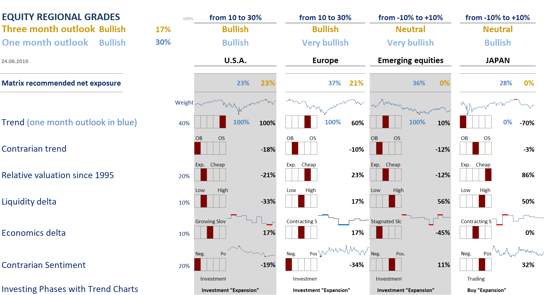
Factor 1: Trend – bullish across all regions
Our underlying philosophy in the construction of this white box is to follow the trend. This is why the Trend and Overbought/Oversold factors have the largest weighting of 40%. The Trend Factor is a moving average model which scores based on the relative movements of price and moving averages of varying durations. The Overbought/Oversold factor aims to add a market timing element to buy low on corrections and sell high on rebounds. The trend indicator is built on data from main market indices across the world, and the calculation is based on a combination of moving averages crossovers. As you can see from the matrix, our trend grades are currently elevated across all regions, ranging from 70% in the US and Europe to the maximum 100% in Japan and EM. To refine this factor, we use an overbought/oversold indicator (our second factor) that either mitigates or amplifies our take on the trend score implies.
The second indicator in our regional matrix provides us with a stance on whether the market is overbought or oversold, suggesting when we might be cautious in the short term and warning us to when to consider cutting or raising our long positions. Currently, this factor suggests very overbought conditions in US.
›The Sentiment factor also contributes to the market timing and is based on our proprietary contrarian PTS sentiment index.
›
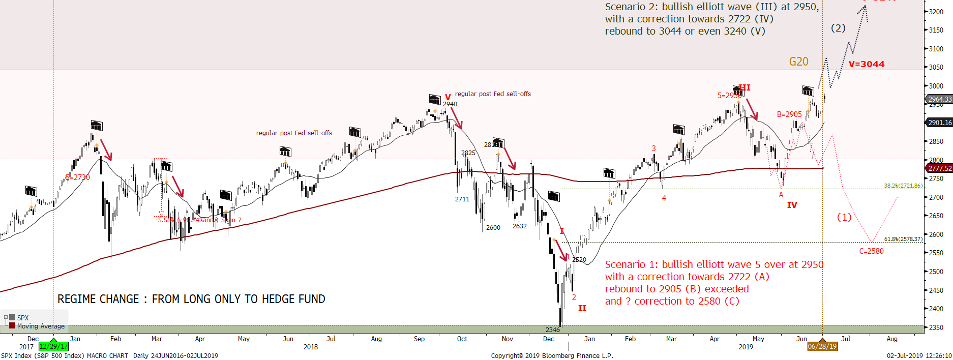
TREND
This adjusted Trend following model is supported by 3 fundamental pillars: the Valuation, Economics and Liquidity factors.
VALUATION
LIQUIDITY
Under the Liquidity label, we want to assess the regional monetary conditions through the yield curve (1), the monetary base changes (2) and central banks’ balance sheets (3) impact. (1) The yield curve is the “Old time” macro predictor. Recessions usually happen in an inverted yield curve environment which occurs when short-term interest rates exceed long-term rates. In the following chart, the yield curve (blue line) IS NEGATIVE BY 47 BPS.
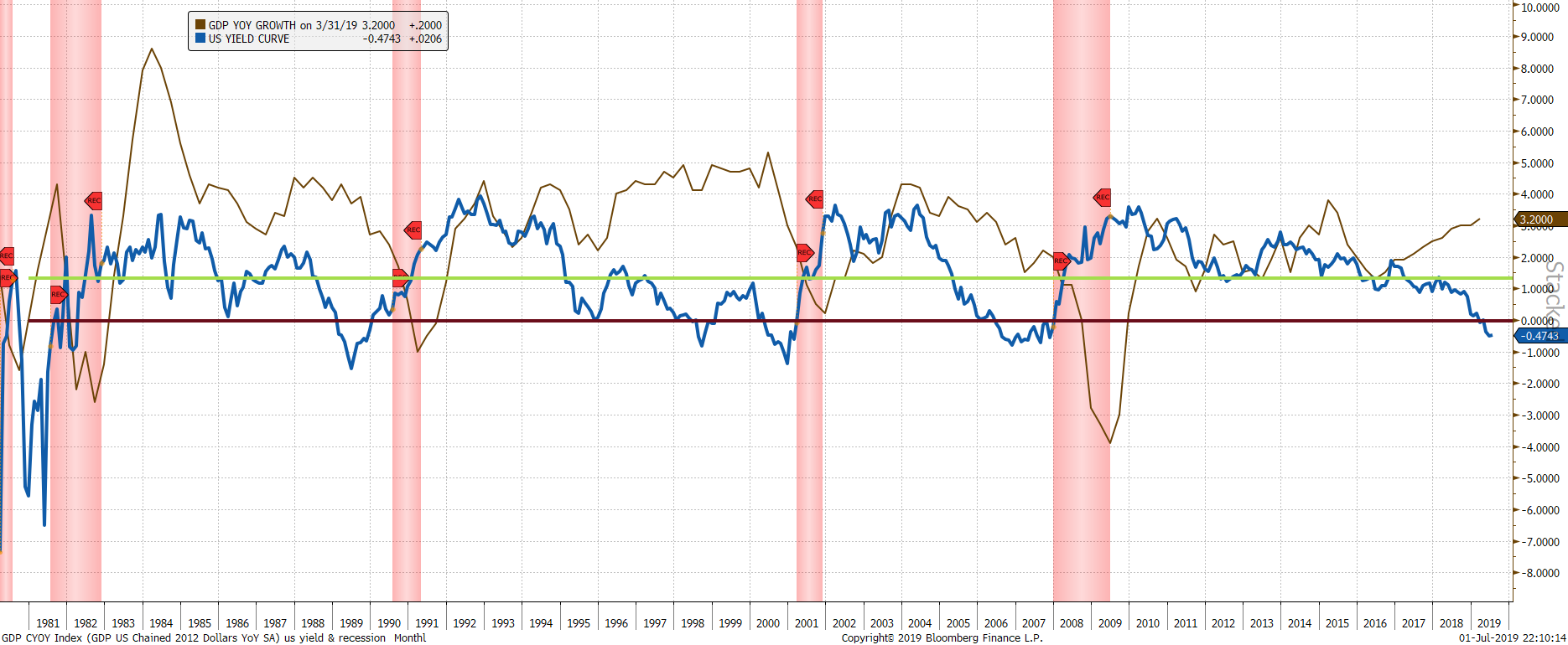
This is a static chart, and a more positive one, the futures curve, as shown below, implies Fed funds will be just 1.32% at year-end 2020, down 106 bps compared to the current rate of 2.38%. If that ptoves to be right and the 10 yar rate stays stable, this should be supportive for risky assets.

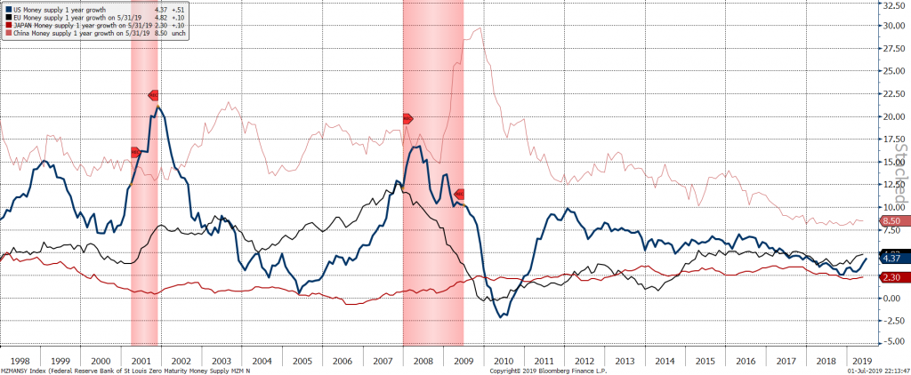
The growth of the money supply is also a major bullish pillar for financial assets. US & Europe exhibit stronger money supply growth since 2018.
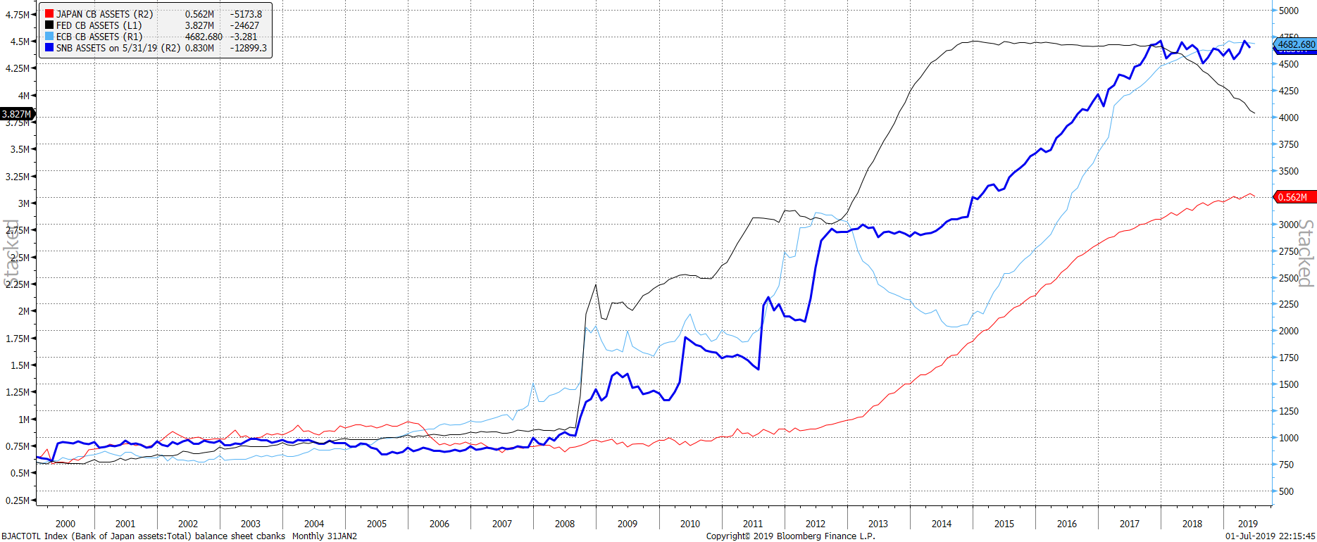
The massive increases of central banks assets (Fed, ECB, BOJ, SNB …) have been a major bullish pillar for financial assets. Only US has ended its QE and thus has a lower liquidity grade then Europe and Japan.
ECONOMICS
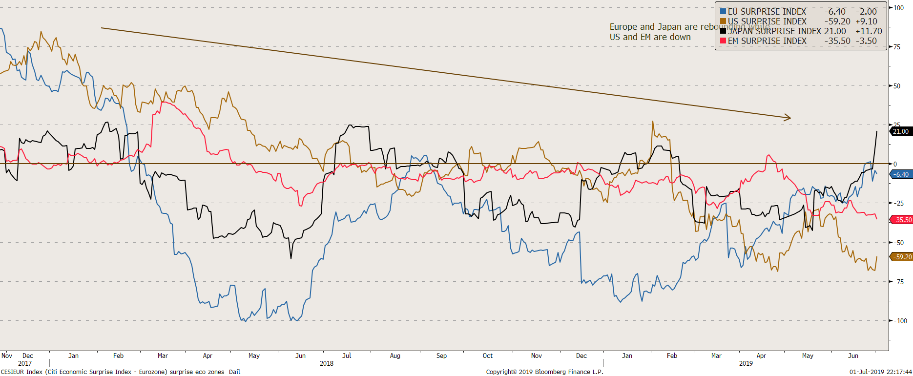
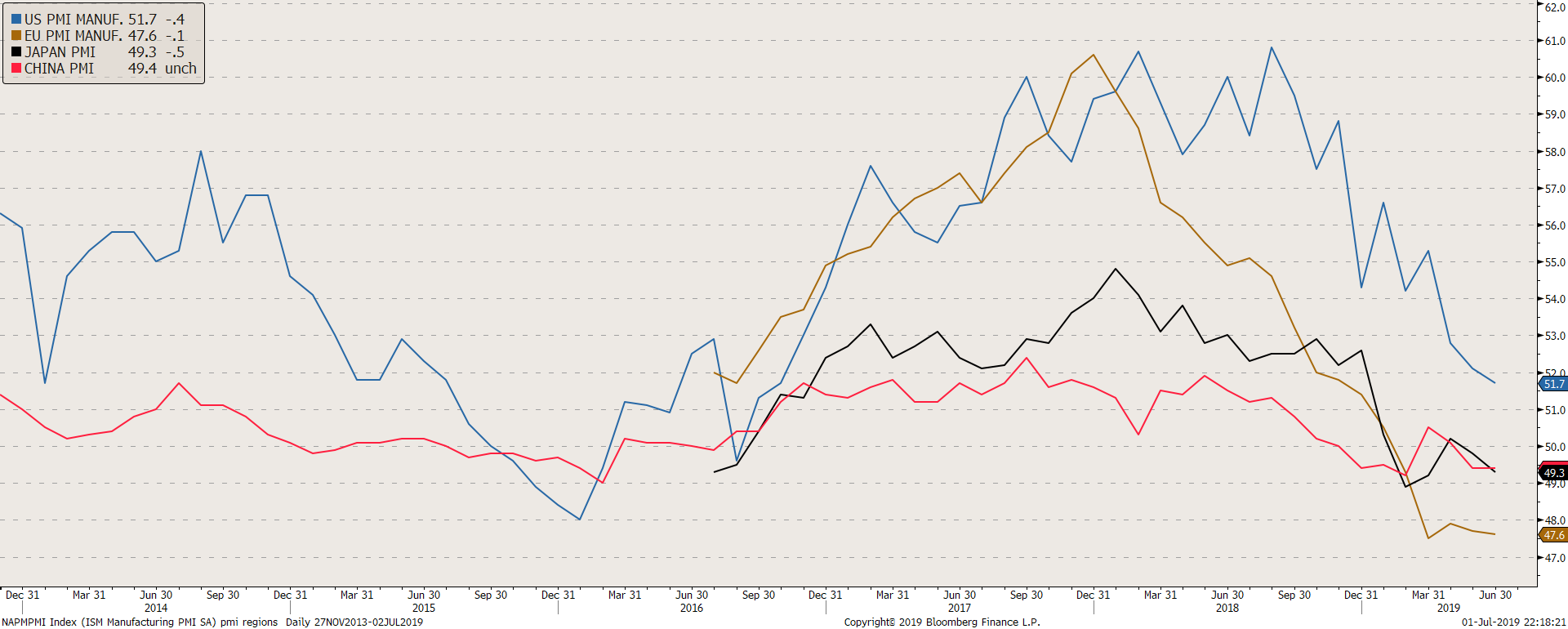
Under the economic label, we want to assess the regional economic conditions through the manufacturing PMI, the non-manufacturing PMI and the economic surprise index. The grade is also ranked from -100% to +100%.
Lingering trade uncertainty has dampened corporate sentiment even further in June. The PPP-weighted global manufacturing PMI fell into contraction territory for the first time since 2016, reaching the lowest level since February 2016. Underlying details were also less encouraging – with new orders now contracting (and well below 2015-16 cycle lows) and the new orders/inventory ratio dipping to a new low since July 2012.
SENTIMENT
Last but not least, the sixth factor is based on a contrarian approach and aims to quantify emotion across the market. When our model identifies sentiment as too confident/fearful, we will reduce/increase our exposure respectively. This strategy works best when it follows the major trend and bets against the immediate shorter term trend. For example, “excessive pessimism” readings will have a very high rate of success preceding rallies during long-term bull markets, but will be less accurate during bear markets. “Excessive optimism” readings will precede corrections with consistency during bear markets, but will be less accurate at pinpointing tops in bull markets.
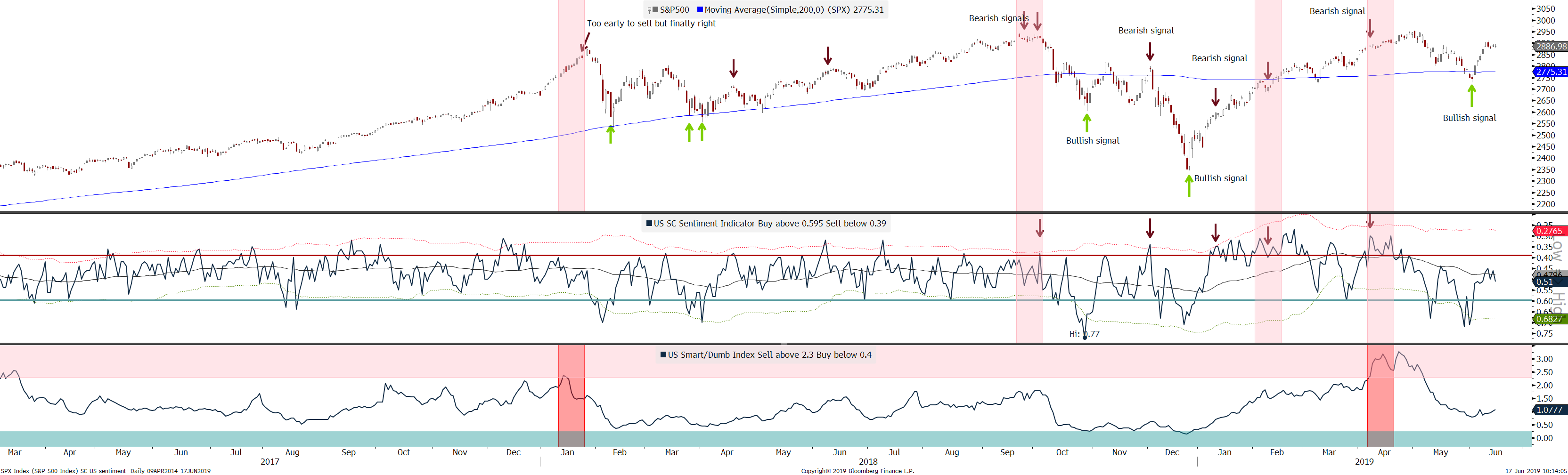
For instance, for the US, we use 2 measures:
<> the PTS sentiment indicator giving very short term contrarian signals (middle chart)
<> the Smart/dumb giving medium run signals (lower hand chart)